In this article, I’m going to explain how to flip a column in Excel 2007, 2010 or 2013 (using screen shots from Excel 2013). Flip a column is what I searched for – you might have asked how to reverse a column or put a column in reverse order.
Note: I was a bit surprised by the solution to this one, but I’ve asked the experts and it is the only way to do this. If you have a better and simpler way (that doesn’t involve macros or coding) please pop a comment on this article or contact me!
Why would I want to put a column in reverse order?
I’m doing my accounts at the moment. I have a spreadsheet of my bank transactions which runs from the newest at the top to the oldest at the bottom. My list of invoices runs from the oldest at the top to the newest at the bottom. If I want to compare them, I want them to both be the same way around, but I need the bank transactions to be in exactly the same order, just the other way around.
Will using Data > Sort flip my column?
The usual way to change the order of columns in Excel is to use the Data > Sort function. However, if you sort by transaction date, it won’t necessarily sort it into the same order the other way around.
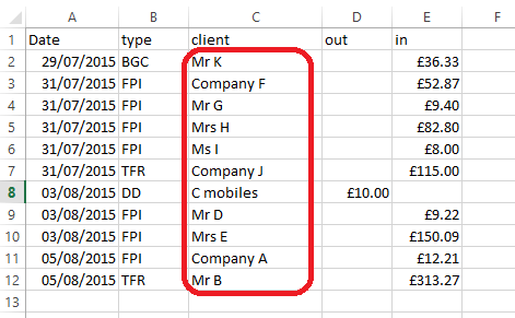
For example, we have a set of bank transactions which I’ve named in alphabetical order down the client column to make it easier to see what happens next:

If I highlight all of the columns, go to the Data tab and choose to sort by date, older to newer, I get this result, which is NOT in exact reverse order:
So, what’s the solution? I was a bit surprised when I searched and searched for the answer, but it is the only way to do it …
So, how do I flip my columns so they’re in exact reverse order?
To do this, we need to create an extra column to sort by, and then reverse sort by that rather than date or any other column.
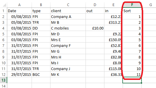
First, create a new column called sort and fill it with numbers from 1 to whatever your total number of rows is:
Expert tip: rather than typing these numbers manually, if you have a lot of rows, and to avoid errors, you can create a quick formula to insert the numbers automatically. Type 1 in the first row then the formula you can see below in the next row, where you get the F2 by clicking on the cell containing the 1:

Then, copy the cell with the formula (right-click, copy), highlight the rest of that column down to the last row and right-click, paste. This will give you the same effect. Note, though, when you sort by this column, the numbers will turn into rows of #####, BUT the sort will still work OK.
Once you have your additional Sort column, you are ready to reverse your columns.
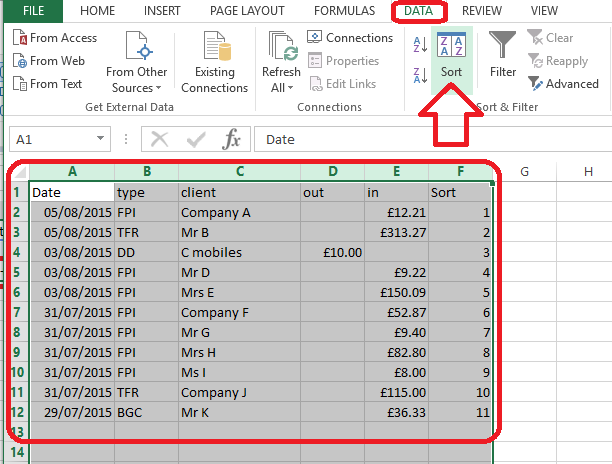
Highlight all of the data and, in the Data Tab, choose Sort:
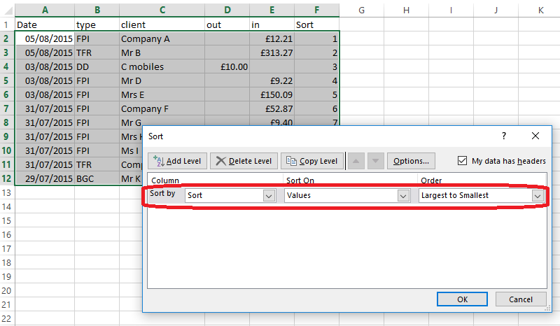
In the Sort Dialog Box, choose to sort by the Sort column, and from Largest to Smallest (i.e. the reverse order to its current order):
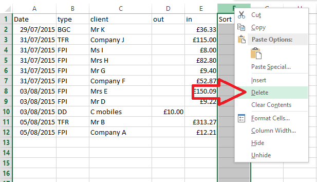
Press OK and hooray – your spreadsheet is sorted into exact reverse order. Just delete the now-redundant Sort column (highlight, right-click, delete):
and here’s your bank transactions in reverse order – you have flipped the column!

This article has explained the (slightly surprising) way to flip the columns in an excel 2007, 2010 or 2013 spreadsheet, not using data sort, but another message. If you need to reverse the order of your columns exactly, then this is the way to do it.
If you’ve found this article helpful or if you have a better solution, please do post a comment below, and if you think others would find it useful, please share it using the sharing buttons below the article. Thank you!
Other useful posts on Excel on this blog:
How to view two workbooks side by side in Excel 2007 and 2010
How to view two pages of a workbook at the same time
How do I print the column headings on every sheet in Excel?
How to print the column and row numbers/ letters and gridlines
Freezing rows and columns in Excel – and freezing both at the same time


