RSS

Category Archives: Excel

Displaying your data in Excel – pivot tables

We can use pivot tables to display the number of times a value appears in a column or row in an Excel spreadsheet.

Why would I use a pivot table to display data?

I keep a record of my reading, including author, publisher, date, fiction or non-fiction, source, if there are any special features like mental health, immigrant experiences etc. I used to tot up some of this information manually using my book blog but this year it’s been in Excel so I can copy other book bloggers and share more detailed information.

I wanted to be able to display numbers of times I read books by x publisher etc. so taught myself this pivot tables / pivot charts procedure.

Setting up a pivot table to display my data counts

Say I want to count the number of times I’ve read books published in particular years in my spreadsheet of books read. I want a graph with the years along the bottom and number of books from each year up the side.

First I select the source data to use, by highlighting the Date column.

Then I go to the Insert tab and select PivotTable then PivotChart:

This brings up a dialogue box. I check the range is in there and then tick the Existing Worksheet option, because I want to display this on my worksheet.

I select the first cell of the destination range to tell it where to paste (I’ve not filled that in yet here), and click OK .

The PivotChart Fields pane appears on the right-hand side of the worksheet. Date (or whatever field you selected) should be showing at the top. Click the tick box next to Date and drag Date down to the Axis section and then the Values section.

The empty Values section populates with Count of Date: this is correct. Once I’ve dragged them down …

As if by magic, a chart appears with my data!

I can move this around and resize it using the arrows that come up as you hover over the box containing the chart.


In this article I’ve shown you how to use pivot tables and pivot charts to make your data display in an easily readable form in Excel.

This works for Excel 2010 and above for PC.

Find other Excel tips in the Excel category!

If you found this article useful, please let me know in a comment!

 
Leave a comment

Posted by on September 25, 2019 in Excel


Tags: , , , ,

How do I search in a whole workbook in Excel?

How do I search for a word or phrase across multiple sheets in a workbook in Excel 2007, 2010, 2013 and 2016?

Why would I want to search a whole workbook?

We think of Excel as being used primarily for numbers (although you might want to search for those, too), but I often encounter spreadsheets full of text. For example, when I’m localising text from US to UK English, or editing text that’s been translated, and it’s been output from a translation tool such as Trados, it often comes to me in an Excel spreadsheet.

Just like when I’m editing a Word or PDF file, I often want to either look for all instances of a word I want to change or check that I haven’t missed anything. And if that word might be in any one of many sheets in a workbook, I will want to search all of those sheets.

How do I perform a search in all the sheets of a workbook?

In this example, I want to find all the instances of the word “authorized” in all the many sheets in an Excel workbook.

First of all, press Control and F at the same time to bring up the Find and Replace dialogue box:

Using this search without changing anything will just search in the sheet I’m currently in.

Click on Options:

This brings up a load of options, including some other exciting ones we’re not looking at here, but which might be useful as well:

Click on the drop-down arrow to the right of Within: Sheet and change it to Workbook:

Now when you click “Find Next”, it will find the cell where that text is throughout the whole workbook.


In this article, we’ve learned how to search a whole workbook in Excel 2007, 2010, 2013 and 2016.

If you’ve found this article helpful, please do post a comment below, and if you think others would find it useful, please share it using the sharing buttons below the article. Thank you!

Other useful posts on Excel on this blog:

How to view two workbooks side by side in Excel 2007 and 2010

How to view two pages of a workbook at the same time

How do I print the column headings on every sheet in Excel?

How to print the column and row numbers/ letters and gridlines

How to change rows into columns and columns into rows in Excel

Freezing rows and columns in Excel – and freezing both at the same time

How to flip a column in Excel – turn it upside down but keep the exact same order!

 
Leave a comment

Posted by on June 20, 2018 in Excel, Short cuts


Tags: , ,

How do I count the number of times a word appears in my document?

I was asked this question during the week, so here’s how to count how many times a particular word appears in a document (or spreadsheet or anything).

The easiest way to count the number of instances of a word is to use the Find function.

Access Find using Control-F (press the control key and F at the same time).

Type in the word you want to search for.

Word will find and highlight all instances of the word and highlight them for you – and will tell you how many times it appears!

Count instances of a word

Note: this search for transcription will find that word buried in other words, too – so TRANSCRIPTIONs and TRANSCRIPTIONist.

To find just the single word transcription, you need to use Advanced Find.

Click on the down arrow next to the search box and then choose Advanced Find:

2 Count instances of a word

Click the More button (which appears where Less is showing here) and then tick the box marked Find Whole Words Only:

3 Count instances of a word

Now Word will count and highlight just the instances of this exact word.

This article has taught you how to count how many times a particular word appears in your document. You can use this method in Excel and PowerPoint, etc. too.

If you’ve found it useful, please click like and share it. Thank you!

Other useful posts on this blog

How to search for anything using Control-F

How to count the words in your Word document

How to count the words in your PowerPoint presentation

Find and Replace

Advanced Find and Replace

 
2 Comments

Posted by on August 3, 2016 in Excel, PowerPoint, Word, Writing


Tags: , , , , ,

How do I change a column into a row or a row into a column in Excel 2007, 2010 and 2013?

In this article, I’m going to explain how to change a column into a row or change a row into a column in Excel 2007, 2010 and 2013 (I think this works in 2016 too but have not yet tested it).

Why would I want to swap a column for a row?

You might start off creating a header row then decide it should be a column, or create a spreadsheet then want to rotate it 90 degrees. Or, worse, someone might decide that for you and expect you know how to do it!

How to change a column into a row or rotate a block of cells

Here’s our original block of cells:

Swap excel rows for columns

We want to turn this around so that everything runs along the top rather than down the side. Here’s how to do it:

First, copy all the cells you want to move:

Highlight the cells, right-click with the mouse, and select Copy:

copying cells in excel

Now, and this is important, find a free, empty cell to paste into. Don’t worry about it being in the middle of the spreadsheet, we will tidy that later.

Right-click with your mouse in an empty cell and then choose Paste Special and Transpose (a hint will appear when you hover over the button, but it’s the one on the bottom right)

How do I swap columns and rows in Excel

Behind all those dialogue boxes, Excel will show you what this is going to look like.

Click on Transpose and your cells will appear, starting from the empty cell you clicked on:

swapped columns and rows

Your original cells are still there – so highlight their columns, right-click with the mouse and choose Delete:

Flipped cells in Excel

And here’s your spreadsheet, the opposite way around from how you started!

5 finished

In this article, we’ve learned how to change rows into columns and change columns into rows in Excel 2007, 2010, 2013 and probably 2016.

If you’ve found this article helpful, please do post a comment below, and if you think others would find it useful, please share it using the sharing buttons below the article. Thank you!

Other useful posts on Excel on this blog:

How to view two workbooks side by side in Excel 2007 and 2010

How to view two pages of a workbook at the same time

How do I print the column headings on every sheet in Excel?

How to print the column and row numbers/ letters and gridlines

Freezing rows and columns in Excel – and freezing both at the same time

How to flip a column in Excel – turn it upside down but keep the exact same order!

 
4 Comments

Posted by on June 8, 2016 in Excel, Short cuts


Tags: , ,

How do I flip a column in Excel 2007, 2010 and 2013?

In this article, I’m going to explain how to flip a column in Excel 2007, 2010 or 2013 (using screen shots from Excel 2013). Flip a column is what I searched for – you might have asked how to reverse a column or put a column in reverse order.

Note: I was a bit surprised by the solution to this one, but I’ve asked the experts and it is the only way to do this. If you have a better and simpler way (that doesn’t involve macros or coding) please pop a comment on this article or contact me!

Why would I want to put a column in reverse order?

I’m doing my accounts at the moment. I have a spreadsheet of my bank transactions which runs from the newest at the top to the oldest at the bottom. My list of invoices runs from the oldest at the top to the newest at the bottom. If I want to compare them, I want them to both be the same way around, but I need the bank transactions to be in exactly the same order, just the other way around.

Will using Data > Sort flip my column?

The usual way to change the order of columns in Excel is to use the Data > Sort function. However, if you sort by transaction date, it won’t necessarily sort it into the same order the other way around.

For example, we have a set of bank transactions which I’ve named in alphabetical order down the client column to make it easier to see what happens next:

1 spreadsheet

If I highlight all of the columns, go to the Data tab and choose to sort by date, older to newer, I get this result, which is NOT in exact reverse order:

1a spreadsheet sorted by date

So, what’s the solution? I was a bit surprised when I searched and searched for the answer, but it is the only way to do it …

So, how do I flip my columns so they’re in exact reverse order?

To do this, we need to create an extra column to sort by, and then reverse sort by that rather than date or any other column.

First, create a new column called sort and fill it with numbers from 1 to whatever your total number of rows is:

2 sort column

Expert tip: rather than typing these numbers manually, if you have a lot of rows, and to avoid errors, you can create a quick formula to insert the numbers automatically. Type 1 in the first row then the formula you can see below in the next row, where you get the F2 by clicking on the cell containing the 1:

2a sort column

Then, copy the cell with the formula (right-click, copy), highlight the rest of that column down to the last row and right-click, paste. This will give you the same effect. Note, though, when you sort by this column, the numbers will turn into rows of #####, BUT the sort will still work OK.

Once you have your additional Sort column, you are ready to reverse your columns.

Highlight all of the data and, in the Data Tab, choose Sort:

4 sort data

In the Sort Dialog Box, choose to sort by the Sort column, and from Largest to Smallest (i.e. the reverse order to its current order):

5 sort data

Press OK and hooray – your spreadsheet is sorted into exact reverse order. Just delete the now-redundant Sort column (highlight, right-click, delete):

7 delete sort column

and here’s your bank transactions in reverse order – you have flipped the column!

6 data sorted

This article has explained the (slightly surprising) way to flip the columns in an excel 2007, 2010 or 2013 spreadsheet, not using data sort, but another message. If you need to reverse the order of your columns exactly, then this is the way to do it.

If you’ve found this article helpful or if you have a better solution, please do post a comment below, and if you think others would find it useful, please share it using the sharing buttons below the article. Thank you!

Other useful posts on Excel on this blog:

How to view two workbooks side by side in Excel 2007 and 2010

How to view two pages of a workbook at the same time

How do I print the column headings on every sheet in Excel?

How to print the column and row numbers/ letters and gridlines

Freezing rows and columns in Excel – and freezing both at the same time

 
6 Comments

Posted by on May 25, 2016 in Excel, Short cuts


Tags: , ,

How do I print the gridlines in my spreadsheet in Excel 2007, 2010 and 2013?

When you’re printing an Excel spreadsheet, how do you make the gridlines print, too?

This article tells you how to print the gridlines automatically, working in the Page Layout Tab, in Excel 2007, 2010 and 2013 (screen shots are taken from Excel 2010).

With your spreadsheet open, go to the Page Layout tab and look to the right to find the Sheet Options area:

print headings

In this area, you can tick Print to make the gridlines appear when you print out the spreadsheet.

There are two things to note here:

  1.  You can also untick the View boxes so you can’t see the gridlines at all. I’m not sure why you might want to do this, but there it is.
  2. If you have used the borders option already to draw borders around some cells, if you print without ticking Print Gridlines, the borders you have added will print anyway; if you tick Print Gridlines, all of the gridlines and borders will print.

Adding customised borders to cells

A quick reminder on adding borders:

Click on the cell(s) you want to add borders to. Click on the Borders drop-down in the Home Tab, Font area:

apply borders excel

then choose where you want your borders to go:

border options excel

More sheet options

You will see that there’s a little arrow in the bottom right corner of the Sheet Options area:

sheet options

Click on this arrow and the Page Setup dialogue box opens – here you can change a few more options, too, or set your headings to print if you want to, as well as going into the other tabs to change the orientation or margins, etc.:

sheet options print gridlines

And that’s it – now you can print the row numbers and heading letters in Excel 2007, 2010 or 2013!

If this has been helpful, please comment below or share the article using the buttons. Thank you!

Related posts on this blog

How do I print the row numbers and column letters in my Excel spreadsheet?

How do I print the Excel header row on every page of my spreadsheet printout?

How do I print the Word header row on every page of my table printout?

 
7 Comments

Posted by on March 23, 2016 in Excel


Tags: , , ,

How do I print row numbers and heading letters in Excel 2007, 2010 and 2013?

When you’re printing an Excel spreadsheet, how do you make the row numbers and heading letters print, too?

This article tells you how to do this, working in the Page Layout Tab, in Excel 2007, 2010 and 2013 (screen shots are taken from Excel 2010).

In your spreadsheet, go to the Page Layout tab and look to the right to find the Sheet Options area:

print headings

In this area, you can tick Print to make the headings (or, indeed, the gridlines) appear when you print out the spreadsheet. Note that if you want to, you can also untick the View boxes so you can’t see the headings. I’m not entirely sure why you wouldn’t want to see those, but the option is there.

You will see that there’s a little arrow in the bottom right corner of the Sheet Options area:

sheet options

Click on this arrow and the Page Setup dialogue box opens – here you can change a few more options, too, or set your headings to print if you want to, as well as going into the other tabs to change the orientation or margins, etc.:

sheet options print headings

And that’s it – now you can print the row numbers and heading letters in Excel 2007, 2010 or 2013!

If this has been helpful, please comment below or share the article using the buttons. Thank you!

Related posts on this blog

How do I print the Excel header row on every page of my spreadsheet printout?

How do I print the Word header row on every page of my table printout?

 
6 Comments

Posted by on March 17, 2016 in Excel


Tags: , , ,

How do I view two sheets of an Excel workbook at the same time?

You’re looking at an Excel spreadsheet workbook which has more than one individual sheet, accessible via clicking on tabs at the bottom of the workbook. This article shows you how to view two different sheets in the same workbook side by side on the page. This article is valid for Excel 2007, Excel 2010 and Excel 2013. It follows on from my article on different ways to view multiple spreadsheets at the same time, and you may wish to refer to that article for further details on the options.

How do I view multiple Excel workbook sheets side by side?

First of all, open up your workbook. You can view different sheets of the workbook by clicking on the tabs at the bottom:

Excel tab to view sheets

However, when you do this, the new sheet is displayed in the window, and you can’t see Sheet1 any more. To be able to view both (or more) at the same time, you will need to create a new window containing the second sheet, and then display them next to each other.

How do I create a new duplicate window in Excel?

First, create a new window. Go into the View tab then click on the New Window button:

Excel new window

This will generate a new window, on top of the first one and identical to it (you can check that you have two open by clicking on the Excel button at the bottom of the screen:

Excel check two files are open

Now, in the window you have just created, click on the tab for the second sheet that you wish to view (in this case, Sheet2):

Excel tab to view sheets

This will display Sheet2 in the new window:

Excel view sheet2

If you want to view more than two sheets, follow this process for each additional sheet that you wish to view.

What are my options for viewing multiple sheets of one workbook in Excel?

Once you’ve got two windows, one displaying the first sheet and one displaying the second, you can view them side by side, or in tiles, or however you choose. In the View tab, click on either View Side by Side or Arrange All to select your options (see this previous article for details on all of the options):

Excel choose options for displaying multiple sheets

Note that if you choose Arrange All, you must make sure that you tick Windows of active workbook:

Excel view multiple sheets active workbook

In this case, I’ve chosen Arrange All – Vertical, and here are my two sheets of my workbook, displayed next to each other:

17 view multiple sheets in a workbook

For details of all of these options and what they do, please see my post on viewing multiple spreadsheets at the same time.

How do I get back to viewing only one sheet at a time?

If you want to return to a full-screen view of a particular spreadsheet, simply double-click on the title bar of your spreadsheet (by its name) and it will expand and be the only one visible:

return to single sheet view

In this article, we’ve learned how to view two or more sheets belonging to one Excel workbook on the screen at the same time, and how to return to a single sheet view.

If you’ve enjoyed this article and found it useful, please take a moment to share it using the buttons below!

Please note, these hints work with versions of Microsoft Excel currently in use – Excel 2007, Excel 2010 and Excel 2013, all for PC. Mac compatible versions of Excel should have similar options. Always save a copy of your document before manipulating it. I bear no responsibility for any pickles you might get yourself into!

Find all the short cuts here … and view the blog resource guide here.

Other useful posts on this blog:

How do I view two Excel spreadsheets at a time?

 
50 Comments

Posted by on September 24, 2014 in Excel, New skills, Short cuts


Tags: , , , , , ,

How do I view two Excel spreadsheets at a time?

You’re looking at a spreadsheet and you want to compare it to another one. In Word, it’s easy to line up two separate documents side by side to look at them both. In Excel – not so easy. This article explains how you can view two Excel spreadsheets next to each other on your screen and compare the two spreadsheets easily (or more, if you want!). Next week, we’re looking at how to view two sheets from the same workbook side by side, too! This article is valid for Excel 2007, Excel 2010 and Excel 2013 to some extent. The problem doesn’t exist in Excel 2013 as you can move spreadsheets around just like you can in Word, however the options still exist for arranging your multiple views (thanks to Alison Lees for pointing out the resolution of the problem).

Why can’t I view two Excel files on the same screen?

If you’re used to working with Word, you’ll know that if you have two Word documents open in any version of Word, you can pick them both up by the top bar (I usually do it near to the name of the document), slide them across to the left and right until they ping back and fill half of the screen …

Two Word documents on one screen

… and end up with two documents next to each other (you can, of course, move the boundary between them to make one bigger and one smaller):

Two Word documents showing side by side

But, if you’ve ever tried to do this with two Excel spreadsheets, you’ll have found that you move one over …

Moving an excel spreadsheet

… and the other one moves to sit underneath it, inaccessible and impossible to view at the same time as, say, Spreadsheet 1:

Second spreadsheet hidden

Move Spreadsheet 2 across to the right and Spreadsheet 1 will follow it. Grrr!

I’m going to show you how you can view both (or even lots of) spreadsheets on the same screen, in various arrangements, and then return to viewing only one. And next week I’ll show you how you can view two sheets from one workbook side by side.

The quick way to view two spreadsheets side by side

We’re going to look at the View tab here. In the View tab, you’ll find a button labelled View Side by Side.

view side by side excel

If you have two spreadsheets open in, say, Excel 2010 (from which these screenshots are taken, but the process is the same for Excel 2007, 2010 and 2013), pressing this button will show you both spreadsheets, one above the other (this always reminds me of playing competitive driving games on the games console):

View side by side - result excel

You can see that the Synchronous Scrolling button is highlighted in the image above. This is a really useful function – if you have both spreadsheets lined up to start with (i.e. you can see Column A and Line 1 at the top left of both), if this button is showing in yellow, scrolling in one spreadsheet (the active one has the scroll bar) will move the other spreadsheet up and down or left and right at the same time:

view side by side synchronous scrolling

However, if you don’t want to use this feature, you can click on the Synchronous Scrolling button to turn it white, and then your two spreadsheets can be scrolled independently (the scroll bar still displays on the active spreadsheet, i.e. the one you’ve clicked on):

view side by side remove synchronous scrolling

Note that synchronous scrolling only works in this View Side by Side option, so if that’s important to you, choose this option.

But what if you want to view the sheets side by side, or more than two in a tiled layout (I’ve got a widescreen monitor so I always want to view side by side)? Read on for that option  …

How do I view two spreadsheets next to each other or in a tiled layout?

To view your multiple spreadsheets arranged next to each other, to swap to the horizontal view we just looked at, or to use the cascade option, stay in the View tab and the same area but click on the Arrange All button:

excel arrange all button

This will give you a range of options for displaying the spreadsheets that you currently have open:

excel arrange all button options

Let’s look at these in turn …

Arrange all – Tiled

If you have two spreadsheets open, the Tiled option in Arrange All will simply show them arranged vertically, i.e. next to each other. All of my other examples feature two spreadsheets, but to demonstrate the Tiled option, here are four spreadsheets:

excel arrange all Tiled option

Note that the spreadsheets arrange themselves in the order in which you have them open, so if Spreadsheet 4 is the last one you looked at, that will appear top left. You can expand and move the individual spreadsheets, then return to Arrange All – Tiled to click them back into position again.

Arrange all – Horizontal

If you choose the Horizontal option in Arrange All, your spreadsheets will appear on top of each other, with the split between them horizontal:

12 arrange all horizontal

Note here that I had Spreadsheet 2 active (visible) when I chose this option, so it appears at the top. To choose which one appears at the top, have that particular spreadsheet visible and active when you click on the Arrange All button.

Arrange All – Vertical

Choosing the Vertical option in Arrange All gives you the two (or more) spreadsheets arranged next to each other, with the split between them vertical:

excel arrange all vertical option

This is how I prefer to view them.

Arrange All – Cascade

I find this one a bit odd. When you choose the Cascade option in Arrange All, the windows containing the individual spreadsheets all appear on top of each other, with a little bit of one poking out from underneath the active one. Here, Spreadsheet 1 is just showing at the top, but if I click on Spreadsheet 1, Spreadsheet 2 will be sticking out at the bottom. It’s odd, but there must be a reason for it, or Excel wouldn’t offer it:

excel arrange all cascade option

How do I get back to viewing only one spreadsheet at a time?

If you want to return to a full-screen view of a particular spreadsheet, simply double-click on the title bar of your spreadsheet (by its name) and it will expand and be the only one visible:

excel return to single sheet view

In this article, we’ve learned how to view two or more Excel spreadsheets on the screen at the same time, and how to return to a single spreadsheet view.

If you’ve enjoyed this article and found it useful, please take a moment to share it using the buttons below!

Please note, these hints work with versions of Microsoft Excel currently in use – Excel 2007, Excel 2010 and Excel 2013, all for PC. Mac compatible versions of Excel should have similar options. Always save a copy of your document before manipulating it. I bear no responsibility for any pickles you might get yourself into!

Find all the short cuts here … and view the blog resource guide here.

 
35 Comments

Posted by on September 17, 2014 in Excel, New skills, Short cuts


Tags: , , , , , ,

How to search for almost anything in Microsoft Office, other software and web pages

Today we’re going to learn about the wonders of Ctrl-F and how it can help you to search for text almost anywhere.

We’re going to look at an overview of the basics in this article, then I’ll go into more detail on advanced searching and replacing in another one.

What does Ctrl-F mean?

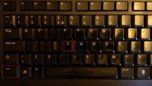
Ctrl-F is shorthand for “press the control key and the F key at the same time“. It’s the way in which key combinations are expressed. You will have one or two Ctrl keys on your keyboard (I have two) and it’s usually easiest to press Ctrl, hold it down, then press F.

keyboard

If you’re looking at a  Word, Excel or Powerpoint document, a web page or, in fact, many other things, you will now be able to search for text in that document, on that page, etc. Let’s go through the different places you can use this.

Searching in Word 2007 using Ctrl-F

Word is one of the places where searching is most useful. It also offers the largest range of options for searching, and we’re just going to look at the most common today but watch this space for an article on advanced searching.

I use Ctrl-F to …

  • Search for a place in a text by a word in its heading
  • Search for tables / figures and references to them in a document to make sure they match up
  • Search for chapter headings in a book / thesis when I want to check they have a consistent style
  • Search for a name to check how it was spelled last time

and many other things.

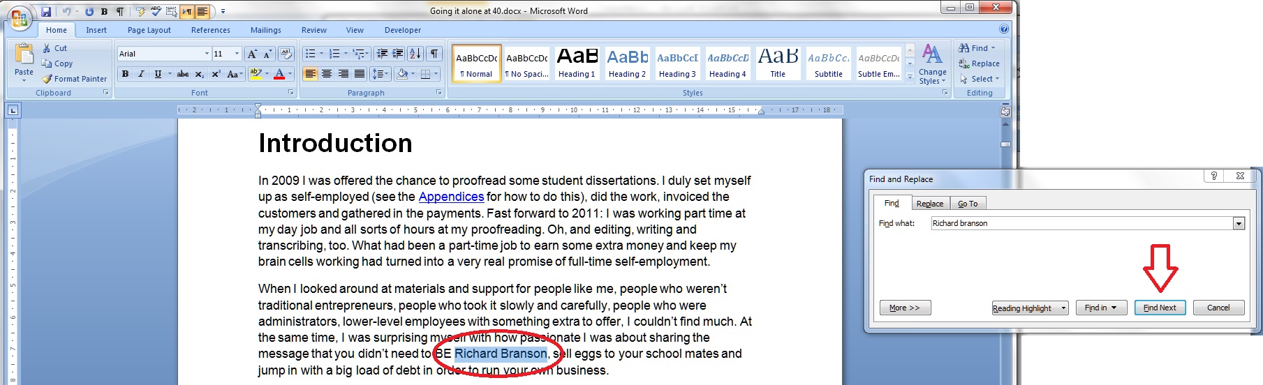
When you have a Word document open, to bring up the search dialogue box, press the Control key and the F key at the same time. You’ll then be presented with the basic search box:

Word 1

It will usually appear to the side of the document, so as not to obscure the text. Enter the text you wish to search for, in this case Richard Branson, and press the Find next button (or the Enter key). Word will highlight the text you’re looking for.

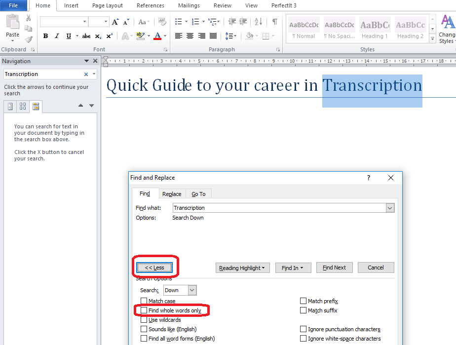
That’s great, but what if you want more accurate searching? Press the More >> button for more options:

Word 2

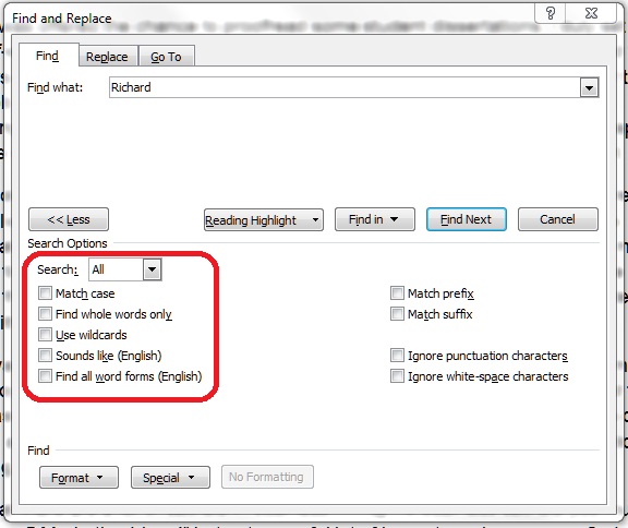
Here, you have options to match the case, find whole words only, etc. For the moment, we’re going to concentrate on just these two (see the article on advanced searching for the other options).

If you choose Match case, it will search for only those words in the exact same case as the one in the search box. If you choose Find whole words only, it will look for only that text, not that text included in a longer word. We’ll have a look at how that works in just a moment.

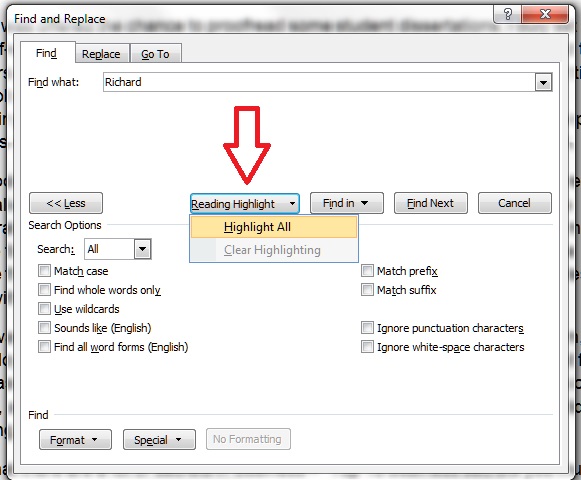
Moving along the options, we have a Reading Highlight button. This will highlight all of the instances of your search word in your document. I find this useful if I’m writing a text to use for Search Engine Optimisation purposes and want to see how many times I’ve included a particular phrase:

Word 3

Note: if you change your search term, you will need to Clear Highlighting before highlighting again, otherwise all of the original highlighting is shown.

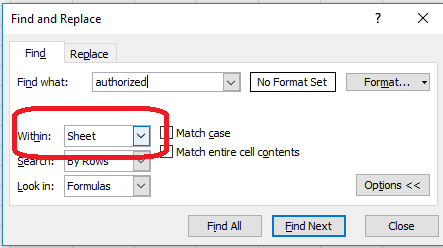
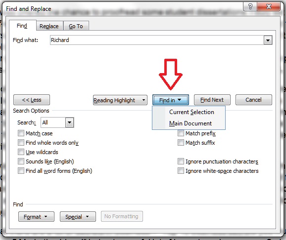
The next option is Find In. This is useful if you only want to search a particular part of the text for your word. Highlight the section in which you want to search, and then choose Current Selection (or, if you’ve got a section highlighted for some other reason, choose Main Document.

Word 4

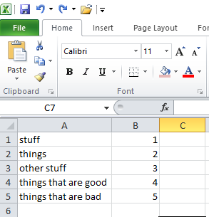
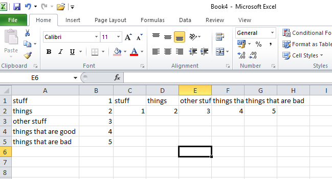
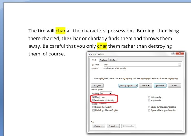
Let’s have a look at some of these options in practice, using a rather odd paragraph I made up for illustration purposes:

Word 5

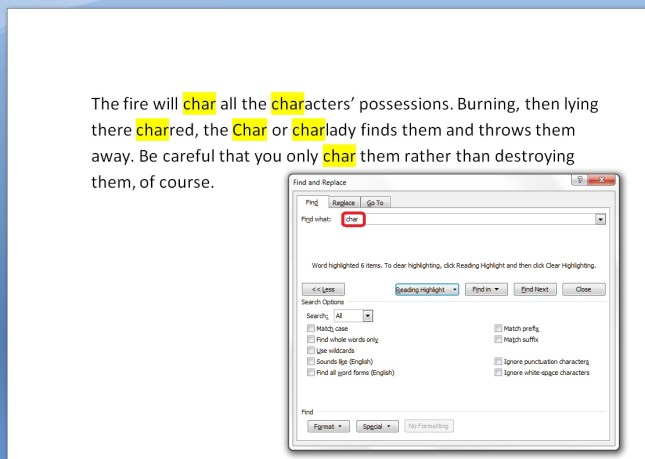
Here, I’ve just searched for char, not worrying about any additional options. You can see that it’s found char, but also character, charlady and Char, because I didn’t specify that I wanted only the word form “char”.

If I want to only find “char” in the text, I need to tell Word to Match case and Find whole words only. Then I will get the desired result:

Word 6

Searching in Word 2010 using Ctrl-F

Of course, they went and changed this to make it more useful and user-friendly in Word 2010 … I was a bit flummoxed when I first tried to use it, but you can get back to the dialogue box we’ve looked at above, and there are some additional useful features.

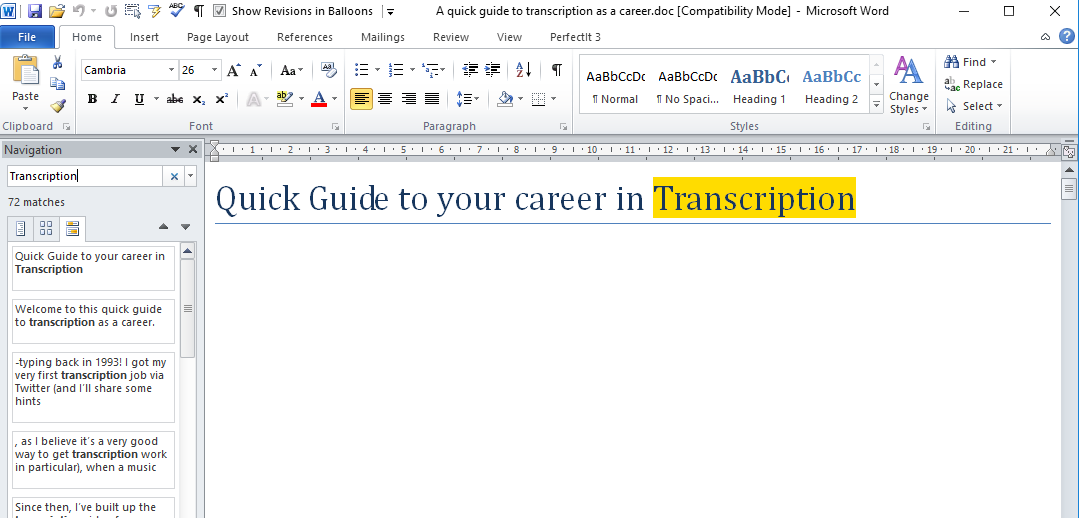
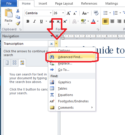
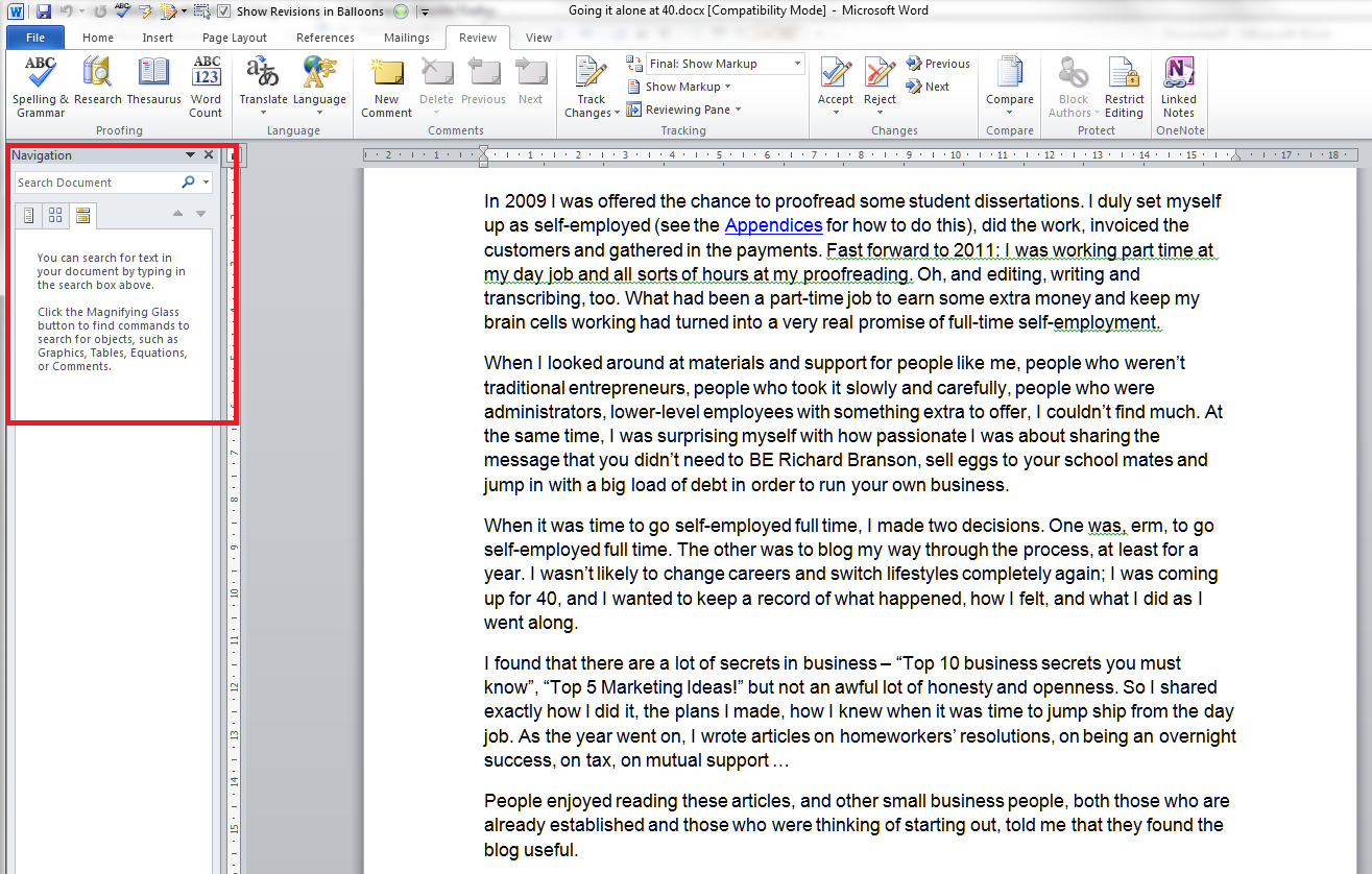
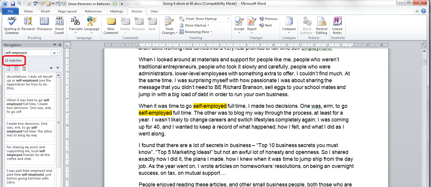
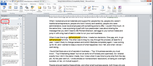
In Word 2010, if you press Ctrl-F, you’ll be given a Navigation pane to the left-hand side of the document:

Word 7

Put your search term in the box and it will automatically highlight all of the instances of that word in the document, give you the number of times it appears, and list all the instances so you can click and visit each of them:

Word 8

This is handy, and although you can do more things here to do with looking at the whole document, you can’t immediately refine your search to whole words only, match case, etc. But you can get to that familiar dialogue box.

Click the down arrow next to the search box and you’ll be presented with a list of options. We’ll look at the advanced ones next time.

Word 9

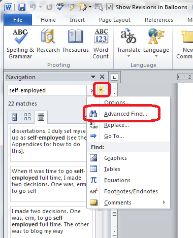
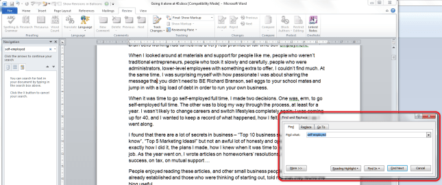
For now, select Advanced Find, and a familiar dialogue box will pop up …

Word 10

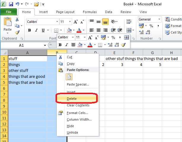
Searching in Excel using Ctrl-F

All of the other software in Microsoft Office uses Ctrl-F, however to a more limited and less customisable degree. In Excel, pressing Ctrl-F will give you this dialogue box:

Excel 1

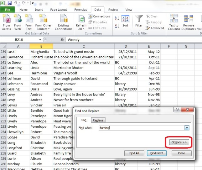
Press the Options button and you have some options for where you search and the form of the word:

Excel 2

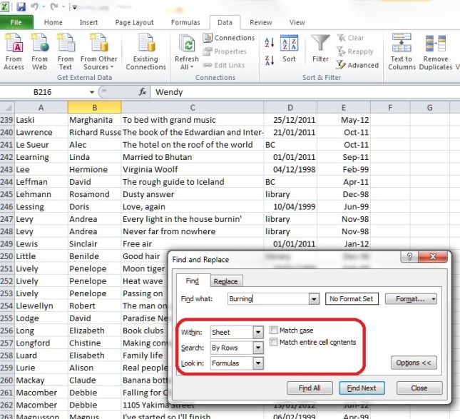
This works the same in Excel 2007 and 2010.

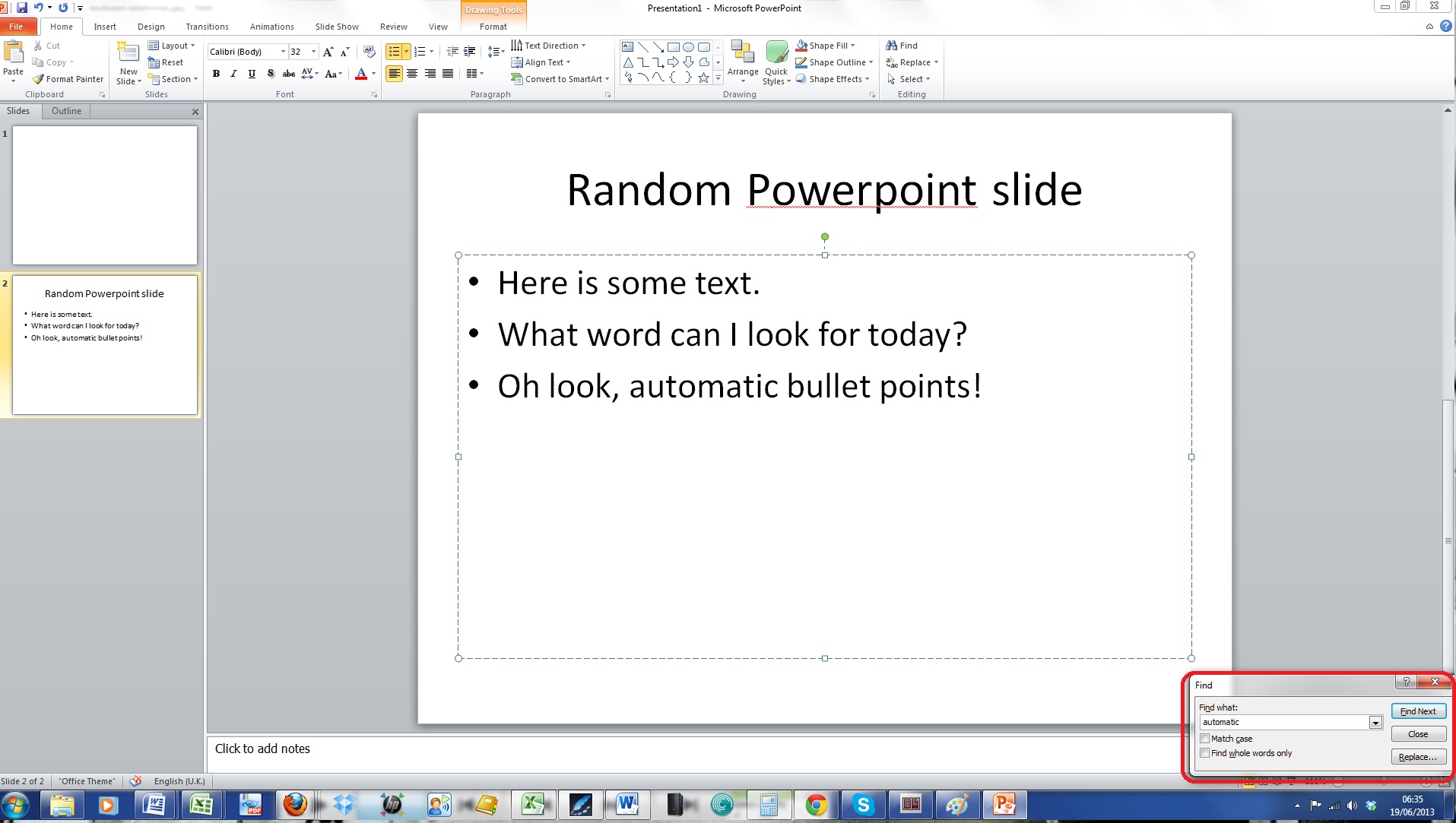
Searching in Powerpoint using Ctrl-F

In Powerpoint, Ctrl-F gives you a small dialogue box:

Powerpoint

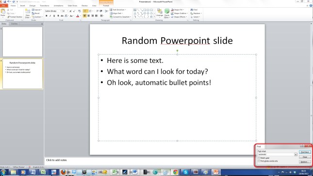
Again, you have enough options to be useful, but not the range of options you find in Word, and again, this works the same in Powerpoint 2007 and 2010.

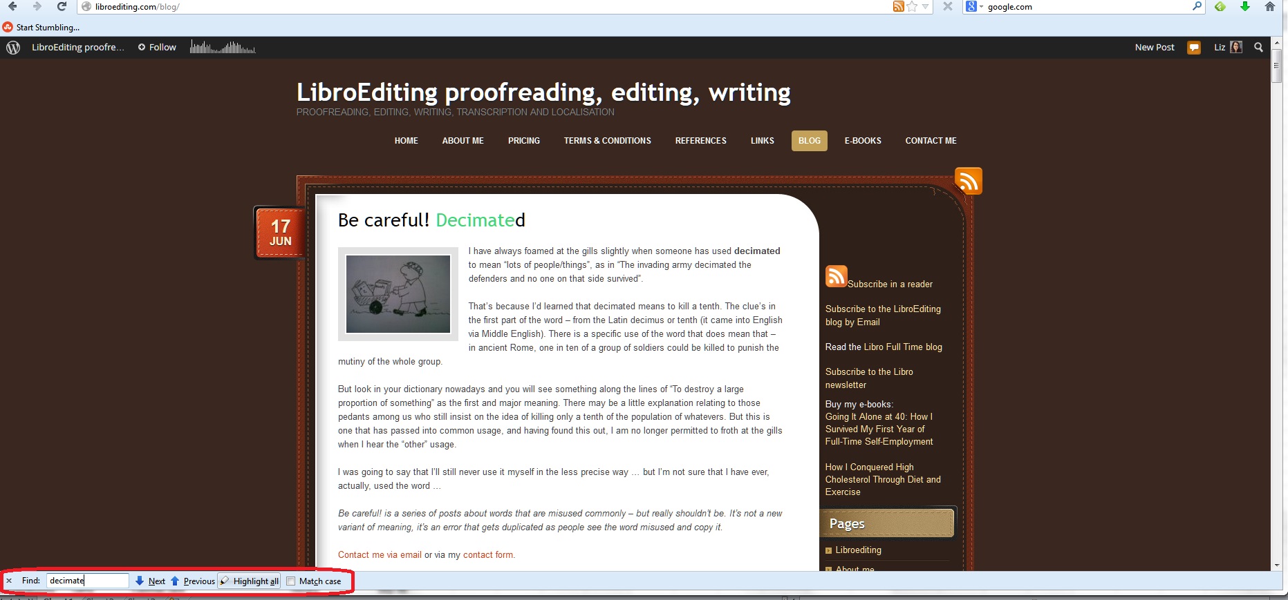
Searching on web pages using Ctrl-F

I find this so useful, especially if I’m searching my own web pages for a word I’ve used or maybe misused (I used this a great deal in the great proof-reading to proofreading change I made a few years ago.

This varies according to the browser you’re using, but hitting Ctrl-F will always bring you up a search box of some kind:

website

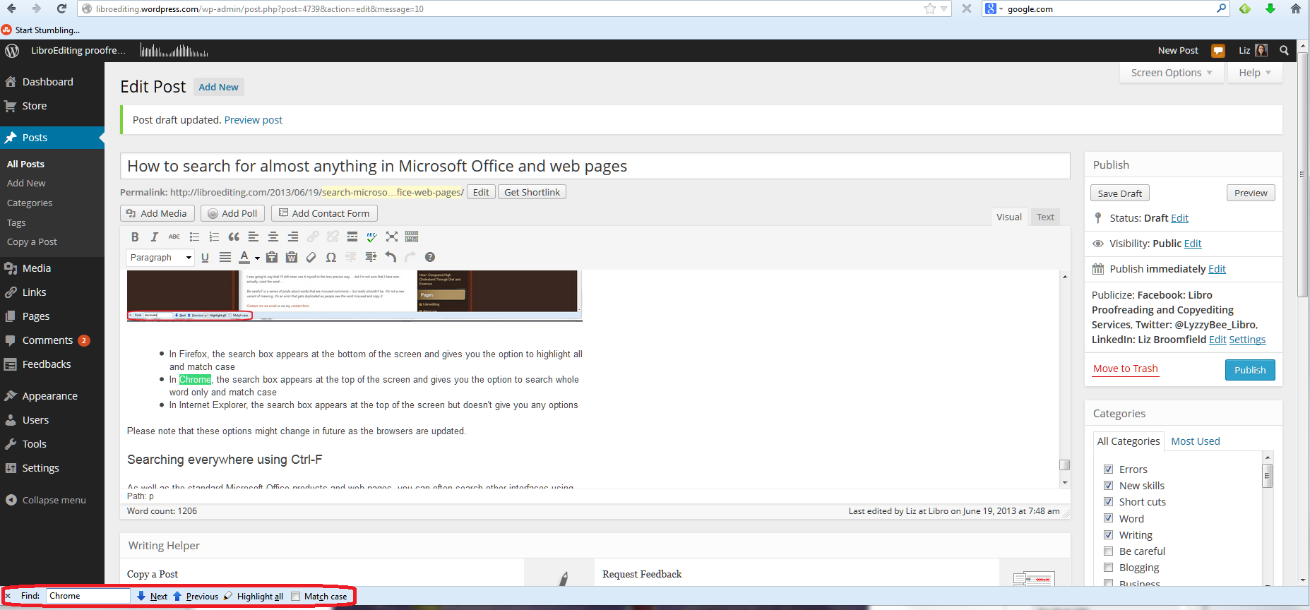
  • In Firefox, the search box appears at the bottom of the screen and gives you the option to highlight all and match case
  • In Chrome, the search box appears at the top of the screen and gives you the option to search whole word only and match case
  • In Internet Explorer, the search box appears at the top of the screen but doesn’t give you any options

Please note that these options might change in future as the browsers are updated.

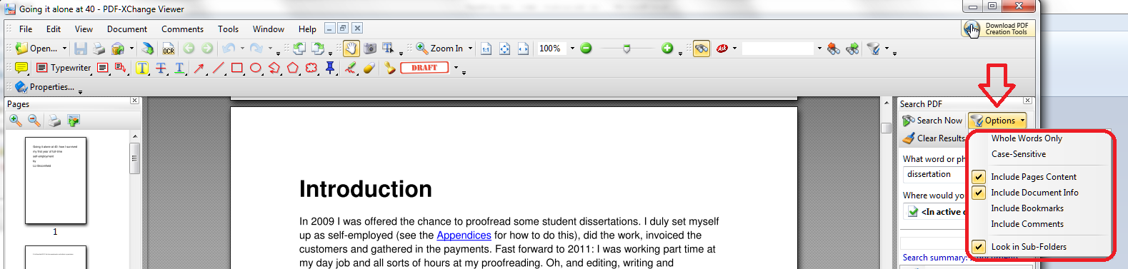
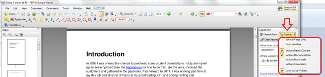
How to search a PDF using Ctrl-F

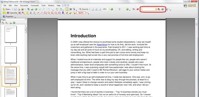
One of the few things that you can’t search using Ctrl-F is a pdf document. However, most readers (I use PDF-Exchange), as well as having their own search functionality on the page, will allow you to use Shift-Ctrl-F to search!

pdf 1

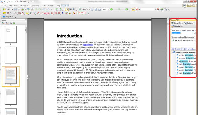
You have some options:

pdf 2

And it works in a similar way in Adobe, too.

If this doesn’t work, there is always a search function in your pdf reader itself, for example:

pdf

Searching anywhere using Ctrl-F

As well as the standard Microsoft Office products and web pages, you can often search other interfaces using Ctrl-F, too. For example, because my WordPress interface uses the web browser, I can search for words in posts I’m writing:

Wordpress

I can use it in Skype:

Skype

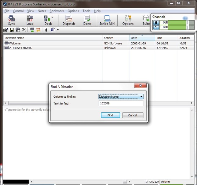
And I’ve even tried it in my transcription management software, ExpressScribe, and you can use it there, too!

express scribe

Today we’ve learned about how to use Ctrl-F to search almost anywhere in any type of document or application.

Coming soon – advanced searching in Word and Search & Replace / Go To.

———————

This is part of my series on how to avoid time-consuming “short cuts” and use Word in the right way to maximise your time and improve the look of your documents.

If you’ve enjoyed this post and/or found it useful, please take a moment to comment (I’ll just ask you to provide a name and email address; you don’t have to sign in to WordPress) and share the post using the buttons you can see below. Thank you!

Please note, these hints work with versions of Microsoft Word currently in use – Word 2003, Word 2007 and Word 2010, all for PC. Mac compatible versions of Word should have similar options. Always save a copy of your document before manipulating it. I bear no responsibility for any pickles you might get yourself into!

Find all the short cuts here


Tags: , , , , , , , ,