RSS

Monthly Archives: September 2014

How do I view two sheets of an Excel workbook at the same time?

You’re looking at an Excel spreadsheet workbook which has more than one individual sheet, accessible via clicking on tabs at the bottom of the workbook. This article shows you how to view two different sheets in the same workbook side by side on the page. This article is valid for Excel 2007, Excel 2010 and Excel 2013. It follows on from my article on different ways to view multiple spreadsheets at the same time, and you may wish to refer to that article for further details on the options.

How do I view multiple Excel workbook sheets side by side?

First of all, open up your workbook. You can view different sheets of the workbook by clicking on the tabs at the bottom:

Excel tab to view sheets

However, when you do this, the new sheet is displayed in the window, and you can’t see Sheet1 any more. To be able to view both (or more) at the same time, you will need to create a new window containing the second sheet, and then display them next to each other.

How do I create a new duplicate window in Excel?

First, create a new window. Go into the View tab then click on the New Window button:

Excel new window

This will generate a new window, on top of the first one and identical to it (you can check that you have two open by clicking on the Excel button at the bottom of the screen:

Excel check two files are open

Now, in the window you have just created, click on the tab for the second sheet that you wish to view (in this case, Sheet2):

Excel tab to view sheets

This will display Sheet2 in the new window:

Excel view sheet2

If you want to view more than two sheets, follow this process for each additional sheet that you wish to view.

What are my options for viewing multiple sheets of one workbook in Excel?

Once you’ve got two windows, one displaying the first sheet and one displaying the second, you can view them side by side, or in tiles, or however you choose. In the View tab, click on either View Side by Side or Arrange All to select your options (see this previous article for details on all of the options):

Excel choose options for displaying multiple sheets

Note that if you choose Arrange All, you must make sure that you tick Windows of active workbook:

Excel view multiple sheets active workbook

In this case, I’ve chosen Arrange All – Vertical, and here are my two sheets of my workbook, displayed next to each other:

17 view multiple sheets in a workbook

For details of all of these options and what they do, please see my post on viewing multiple spreadsheets at the same time.

How do I get back to viewing only one sheet at a time?

If you want to return to a full-screen view of a particular spreadsheet, simply double-click on the title bar of your spreadsheet (by its name) and it will expand and be the only one visible:

return to single sheet view

In this article, we’ve learned how to view two or more sheets belonging to one Excel workbook on the screen at the same time, and how to return to a single sheet view.

If you’ve enjoyed this article and found it useful, please take a moment to share it using the buttons below!

Please note, these hints work with versions of Microsoft Excel currently in use – Excel 2007, Excel 2010 and Excel 2013, all for PC. Mac compatible versions of Excel should have similar options. Always save a copy of your document before manipulating it. I bear no responsibility for any pickles you might get yourself into!

Find all the short cuts here … and view the blog resource guide here.

Other useful posts on this blog:

How do I view two Excel spreadsheets at a time?

 
50 Comments

Posted by on September 24, 2014 in Excel, New skills, Short cuts


Tags: , , , , , ,

How do I view two Excel spreadsheets at a time?

You’re looking at a spreadsheet and you want to compare it to another one. In Word, it’s easy to line up two separate documents side by side to look at them both. In Excel – not so easy. This article explains how you can view two Excel spreadsheets next to each other on your screen and compare the two spreadsheets easily (or more, if you want!). Next week, we’re looking at how to view two sheets from the same workbook side by side, too! This article is valid for Excel 2007, Excel 2010 and Excel 2013 to some extent. The problem doesn’t exist in Excel 2013 as you can move spreadsheets around just like you can in Word, however the options still exist for arranging your multiple views (thanks to Alison Lees for pointing out the resolution of the problem).

Why can’t I view two Excel files on the same screen?

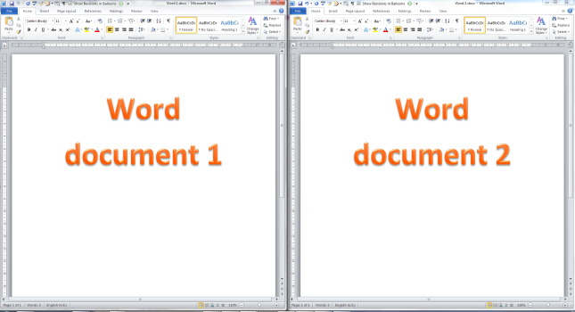
If you’re used to working with Word, you’ll know that if you have two Word documents open in any version of Word, you can pick them both up by the top bar (I usually do it near to the name of the document), slide them across to the left and right until they ping back and fill half of the screen …

Two Word documents on one screen

… and end up with two documents next to each other (you can, of course, move the boundary between them to make one bigger and one smaller):

Two Word documents showing side by side

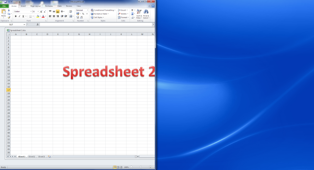
But, if you’ve ever tried to do this with two Excel spreadsheets, you’ll have found that you move one over …

Moving an excel spreadsheet

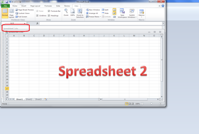
… and the other one moves to sit underneath it, inaccessible and impossible to view at the same time as, say, Spreadsheet 1:

Second spreadsheet hidden

Move Spreadsheet 2 across to the right and Spreadsheet 1 will follow it. Grrr!

I’m going to show you how you can view both (or even lots of) spreadsheets on the same screen, in various arrangements, and then return to viewing only one. And next week I’ll show you how you can view two sheets from one workbook side by side.

The quick way to view two spreadsheets side by side

We’re going to look at the View tab here. In the View tab, you’ll find a button labelled View Side by Side.

view side by side excel

If you have two spreadsheets open in, say, Excel 2010 (from which these screenshots are taken, but the process is the same for Excel 2007, 2010 and 2013), pressing this button will show you both spreadsheets, one above the other (this always reminds me of playing competitive driving games on the games console):

View side by side - result excel

You can see that the Synchronous Scrolling button is highlighted in the image above. This is a really useful function – if you have both spreadsheets lined up to start with (i.e. you can see Column A and Line 1 at the top left of both), if this button is showing in yellow, scrolling in one spreadsheet (the active one has the scroll bar) will move the other spreadsheet up and down or left and right at the same time:

view side by side synchronous scrolling

However, if you don’t want to use this feature, you can click on the Synchronous Scrolling button to turn it white, and then your two spreadsheets can be scrolled independently (the scroll bar still displays on the active spreadsheet, i.e. the one you’ve clicked on):

view side by side remove synchronous scrolling

Note that synchronous scrolling only works in this View Side by Side option, so if that’s important to you, choose this option.

But what if you want to view the sheets side by side, or more than two in a tiled layout (I’ve got a widescreen monitor so I always want to view side by side)? Read on for that option  …

How do I view two spreadsheets next to each other or in a tiled layout?

To view your multiple spreadsheets arranged next to each other, to swap to the horizontal view we just looked at, or to use the cascade option, stay in the View tab and the same area but click on the Arrange All button:

excel arrange all button

This will give you a range of options for displaying the spreadsheets that you currently have open:

excel arrange all button options

Let’s look at these in turn …

Arrange all – Tiled

If you have two spreadsheets open, the Tiled option in Arrange All will simply show them arranged vertically, i.e. next to each other. All of my other examples feature two spreadsheets, but to demonstrate the Tiled option, here are four spreadsheets:

excel arrange all Tiled option

Note that the spreadsheets arrange themselves in the order in which you have them open, so if Spreadsheet 4 is the last one you looked at, that will appear top left. You can expand and move the individual spreadsheets, then return to Arrange All – Tiled to click them back into position again.

Arrange all – Horizontal

If you choose the Horizontal option in Arrange All, your spreadsheets will appear on top of each other, with the split between them horizontal:

12 arrange all horizontal

Note here that I had Spreadsheet 2 active (visible) when I chose this option, so it appears at the top. To choose which one appears at the top, have that particular spreadsheet visible and active when you click on the Arrange All button.

Arrange All – Vertical

Choosing the Vertical option in Arrange All gives you the two (or more) spreadsheets arranged next to each other, with the split between them vertical:

excel arrange all vertical option

This is how I prefer to view them.

Arrange All – Cascade

I find this one a bit odd. When you choose the Cascade option in Arrange All, the windows containing the individual spreadsheets all appear on top of each other, with a little bit of one poking out from underneath the active one. Here, Spreadsheet 1 is just showing at the top, but if I click on Spreadsheet 1, Spreadsheet 2 will be sticking out at the bottom. It’s odd, but there must be a reason for it, or Excel wouldn’t offer it:

excel arrange all cascade option

How do I get back to viewing only one spreadsheet at a time?

If you want to return to a full-screen view of a particular spreadsheet, simply double-click on the title bar of your spreadsheet (by its name) and it will expand and be the only one visible:

excel return to single sheet view

In this article, we’ve learned how to view two or more Excel spreadsheets on the screen at the same time, and how to return to a single spreadsheet view.

If you’ve enjoyed this article and found it useful, please take a moment to share it using the buttons below!

Please note, these hints work with versions of Microsoft Excel currently in use – Excel 2007, Excel 2010 and Excel 2013, all for PC. Mac compatible versions of Excel should have similar options. Always save a copy of your document before manipulating it. I bear no responsibility for any pickles you might get yourself into!

Find all the short cuts here … and view the blog resource guide here.

 
35 Comments

Posted by on September 17, 2014 in Excel, New skills, Short cuts


Tags: , , , , , ,

How to avoid two common mistakes when using MailChimp

Mailchimp is a very popular program for sending newsletters – mainly because it’s free to use to send newsletters and other messages to up to 12,000 emails per month to up to 2,000 subscribers. I use it myself, as do the people who write quite a few of the newsletters I subscribe to. If you use MailChimp yourself, this post helps you to avoid two common mistakes that I see occurring very frequently (and if you don’t use it yourself, I bet you see at least one of these in the newsletters you subscribe to – feel free to share this post with their creators!).

What am I talking about?

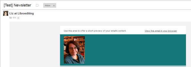
Well, this is what you might see in your email box when you receive a newsletter:

MailChimp newsletter email with errors

Ignore the “[Test]” – that’s me sending test copies of my newsletter to myself for demonstration purposes. So, with email on preview mode, and then when you open the email:

Full MailChimp email with errors

… what can we see here?

  1. The email subject is simply “Newsletter”. Not that inviting.
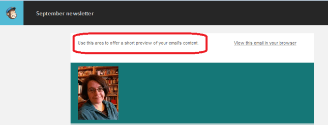
  2. This is the biggie – there’s an odd bit of text in the preview that reads “Use this area to offer a short preview of your email’s content.”

How often have you seen the second point and been confused or even tutted slightly to yourself? (Note: as a kind editor, I avoid tutting. But I do smile wryly every time I see it and think, “I really MUST write a blog post about that one”).

How do these MailChimp mistakes come about?

I’m going to assume here that you know how to set up and send a MailChimp newsletter campaign, and just concentrate on eliminating these errors. If you need a step-by-step MailChimp walkthrough, let me know in the comments and I’ll put one together for you if enough people want it.

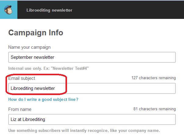
The boring email title error comes on the Campaign Info page:

MailChimp campaign info pageIf you set up your very first campaign with a title like this, it will carry on sending it like that forever, but this is editable. I’m not going to go into ideas for good subject lines here – first off, MailChimp obviously provides a link to some further information, as you can see from the screenshot, but I’d like to take a moment here to mention my client Nathan Littleton’s book, “Delivered“, which has masses of information on creating a good email marketing campaign, including lots of advice on subject lines (he’s not sponsoring this post: I edited this book and I got loads of ideas from it which I’ve implemented in my own newsletter, to good effect).

So, first things first: change that Email subject field to a good, interesting phrase and I’d like to bet that you’ll stop boring your subscriber list and get more opens.

The second one is the dreaded “Use this area … ” text. How does it get there?

Well, when you get to the Design screen in your campaign creation process, bits of helpful text automatically appear in your template to tell you what to do. And one of the bits of helpful text that always appears is this one, right in the top of the screen, and in ever such a small font so that you’re very likely not to see it:

Sample teaser text in MailChimp

And that’s where that text pulls from that displays in your recipients’ emails.

Whatever the design, it’s always up there. Your eye is of course drawn to the main body of the email – the nice picture, the lovingly crafted text you’re going to place into the template.

What do you need to do here? Simply click on that teaser text, just like you would to edit the main body of the newsletter, and you can enter whatever text you want to.

What should it look like?

Once you’ve given your newsletter a more dynamic subject line and eradicated that bit of pesky sample text, this is what your email recipients will see:

MailChimp errors corrected

I think you’ll agree that you’d be more likely to open that one .. and so will your newsletter recipients!

In this article I’ve shared how to avoid two common MailChimp newsletter errors. Please do use the sharing buttons below to share this with anyone who you think might find it useful – thank you!

 
48 Comments

Posted by on September 10, 2014 in Business, Errors, Social media


Tags: , ,