RSS

Tag Archives: Excel2010

Displaying your data in Excel – pivot tables

We can use pivot tables to display the number of times a value appears in a column or row in an Excel spreadsheet.

Why would I use a pivot table to display data?

I keep a record of my reading, including author, publisher, date, fiction or non-fiction, source, if there are any special features like mental health, immigrant experiences etc. I used to tot up some of this information manually using my book blog but this year it’s been in Excel so I can copy other book bloggers and share more detailed information.

I wanted to be able to display numbers of times I read books by x publisher etc. so taught myself this pivot tables / pivot charts procedure.

Setting up a pivot table to display my data counts

Say I want to count the number of times I’ve read books published in particular years in my spreadsheet of books read. I want a graph with the years along the bottom and number of books from each year up the side.

First I select the source data to use, by highlighting the Date column.

Then I go to the Insert tab and select PivotTable then PivotChart:

This brings up a dialogue box. I check the range is in there and then tick the Existing Worksheet option, because I want to display this on my worksheet.

I select the first cell of the destination range to tell it where to paste (I’ve not filled that in yet here), and click OK .

The PivotChart Fields pane appears on the right-hand side of the worksheet. Date (or whatever field you selected) should be showing at the top. Click the tick box next to Date and drag Date down to the Axis section and then the Values section.

The empty Values section populates with Count of Date: this is correct. Once I’ve dragged them down …

As if by magic, a chart appears with my data!

I can move this around and resize it using the arrows that come up as you hover over the box containing the chart.


In this article I’ve shown you how to use pivot tables and pivot charts to make your data display in an easily readable form in Excel.

This works for Excel 2010 and above for PC.

Find other Excel tips in the Excel category!

If you found this article useful, please let me know in a comment!

 
Leave a comment

Posted by on September 25, 2019 in Excel


Tags: , , , ,

How do I print the gridlines in my spreadsheet in Excel 2007, 2010 and 2013?

When you’re printing an Excel spreadsheet, how do you make the gridlines print, too?

This article tells you how to print the gridlines automatically, working in the Page Layout Tab, in Excel 2007, 2010 and 2013 (screen shots are taken from Excel 2010).

With your spreadsheet open, go to the Page Layout tab and look to the right to find the Sheet Options area:

print headings

In this area, you can tick Print to make the gridlines appear when you print out the spreadsheet.

There are two things to note here:

  1.  You can also untick the View boxes so you can’t see the gridlines at all. I’m not sure why you might want to do this, but there it is.
  2. If you have used the borders option already to draw borders around some cells, if you print without ticking Print Gridlines, the borders you have added will print anyway; if you tick Print Gridlines, all of the gridlines and borders will print.

Adding customised borders to cells

A quick reminder on adding borders:

Click on the cell(s) you want to add borders to. Click on the Borders drop-down in the Home Tab, Font area:

apply borders excel

then choose where you want your borders to go:

border options excel

More sheet options

You will see that there’s a little arrow in the bottom right corner of the Sheet Options area:

sheet options

Click on this arrow and the Page Setup dialogue box opens – here you can change a few more options, too, or set your headings to print if you want to, as well as going into the other tabs to change the orientation or margins, etc.:

sheet options print gridlines

And that’s it – now you can print the row numbers and heading letters in Excel 2007, 2010 or 2013!

If this has been helpful, please comment below or share the article using the buttons. Thank you!

Related posts on this blog

How do I print the row numbers and column letters in my Excel spreadsheet?

How do I print the Excel header row on every page of my spreadsheet printout?

How do I print the Word header row on every page of my table printout?

 
7 Comments

Posted by on March 23, 2016 in Excel


Tags: , , ,

How do I print row numbers and heading letters in Excel 2007, 2010 and 2013?

When you’re printing an Excel spreadsheet, how do you make the row numbers and heading letters print, too?

This article tells you how to do this, working in the Page Layout Tab, in Excel 2007, 2010 and 2013 (screen shots are taken from Excel 2010).

In your spreadsheet, go to the Page Layout tab and look to the right to find the Sheet Options area:

print headings

In this area, you can tick Print to make the headings (or, indeed, the gridlines) appear when you print out the spreadsheet. Note that if you want to, you can also untick the View boxes so you can’t see the headings. I’m not entirely sure why you wouldn’t want to see those, but the option is there.

You will see that there’s a little arrow in the bottom right corner of the Sheet Options area:

sheet options

Click on this arrow and the Page Setup dialogue box opens – here you can change a few more options, too, or set your headings to print if you want to, as well as going into the other tabs to change the orientation or margins, etc.:

sheet options print headings

And that’s it – now you can print the row numbers and heading letters in Excel 2007, 2010 or 2013!

If this has been helpful, please comment below or share the article using the buttons. Thank you!

Related posts on this blog

How do I print the Excel header row on every page of my spreadsheet printout?

How do I print the Word header row on every page of my table printout?

 
6 Comments

Posted by on March 17, 2016 in Excel


Tags: , , ,

How do I view two sheets of an Excel workbook at the same time?

You’re looking at an Excel spreadsheet workbook which has more than one individual sheet, accessible via clicking on tabs at the bottom of the workbook. This article shows you how to view two different sheets in the same workbook side by side on the page. This article is valid for Excel 2007, Excel 2010 and Excel 2013. It follows on from my article on different ways to view multiple spreadsheets at the same time, and you may wish to refer to that article for further details on the options.

How do I view multiple Excel workbook sheets side by side?

First of all, open up your workbook. You can view different sheets of the workbook by clicking on the tabs at the bottom:

Excel tab to view sheets

However, when you do this, the new sheet is displayed in the window, and you can’t see Sheet1 any more. To be able to view both (or more) at the same time, you will need to create a new window containing the second sheet, and then display them next to each other.

How do I create a new duplicate window in Excel?

First, create a new window. Go into the View tab then click on the New Window button:

Excel new window

This will generate a new window, on top of the first one and identical to it (you can check that you have two open by clicking on the Excel button at the bottom of the screen:

Excel check two files are open

Now, in the window you have just created, click on the tab for the second sheet that you wish to view (in this case, Sheet2):

Excel tab to view sheets

This will display Sheet2 in the new window:

Excel view sheet2

If you want to view more than two sheets, follow this process for each additional sheet that you wish to view.

What are my options for viewing multiple sheets of one workbook in Excel?

Once you’ve got two windows, one displaying the first sheet and one displaying the second, you can view them side by side, or in tiles, or however you choose. In the View tab, click on either View Side by Side or Arrange All to select your options (see this previous article for details on all of the options):

Excel choose options for displaying multiple sheets

Note that if you choose Arrange All, you must make sure that you tick Windows of active workbook:

Excel view multiple sheets active workbook

In this case, I’ve chosen Arrange All – Vertical, and here are my two sheets of my workbook, displayed next to each other:

17 view multiple sheets in a workbook

For details of all of these options and what they do, please see my post on viewing multiple spreadsheets at the same time.

How do I get back to viewing only one sheet at a time?

If you want to return to a full-screen view of a particular spreadsheet, simply double-click on the title bar of your spreadsheet (by its name) and it will expand and be the only one visible:

return to single sheet view

In this article, we’ve learned how to view two or more sheets belonging to one Excel workbook on the screen at the same time, and how to return to a single sheet view.

If you’ve enjoyed this article and found it useful, please take a moment to share it using the buttons below!

Please note, these hints work with versions of Microsoft Excel currently in use – Excel 2007, Excel 2010 and Excel 2013, all for PC. Mac compatible versions of Excel should have similar options. Always save a copy of your document before manipulating it. I bear no responsibility for any pickles you might get yourself into!

Find all the short cuts here … and view the blog resource guide here.

Other useful posts on this blog:

How do I view two Excel spreadsheets at a time?

 
50 Comments

Posted by on September 24, 2014 in Excel, New skills, Short cuts


Tags: , , , , , ,

How do I view two Excel spreadsheets at a time?

You’re looking at a spreadsheet and you want to compare it to another one. In Word, it’s easy to line up two separate documents side by side to look at them both. In Excel – not so easy. This article explains how you can view two Excel spreadsheets next to each other on your screen and compare the two spreadsheets easily (or more, if you want!). Next week, we’re looking at how to view two sheets from the same workbook side by side, too! This article is valid for Excel 2007, Excel 2010 and Excel 2013 to some extent. The problem doesn’t exist in Excel 2013 as you can move spreadsheets around just like you can in Word, however the options still exist for arranging your multiple views (thanks to Alison Lees for pointing out the resolution of the problem).

Why can’t I view two Excel files on the same screen?

If you’re used to working with Word, you’ll know that if you have two Word documents open in any version of Word, you can pick them both up by the top bar (I usually do it near to the name of the document), slide them across to the left and right until they ping back and fill half of the screen …

Two Word documents on one screen

… and end up with two documents next to each other (you can, of course, move the boundary between them to make one bigger and one smaller):

Two Word documents showing side by side

But, if you’ve ever tried to do this with two Excel spreadsheets, you’ll have found that you move one over …

Moving an excel spreadsheet

… and the other one moves to sit underneath it, inaccessible and impossible to view at the same time as, say, Spreadsheet 1:

Second spreadsheet hidden

Move Spreadsheet 2 across to the right and Spreadsheet 1 will follow it. Grrr!

I’m going to show you how you can view both (or even lots of) spreadsheets on the same screen, in various arrangements, and then return to viewing only one. And next week I’ll show you how you can view two sheets from one workbook side by side.

The quick way to view two spreadsheets side by side

We’re going to look at the View tab here. In the View tab, you’ll find a button labelled View Side by Side.

view side by side excel

If you have two spreadsheets open in, say, Excel 2010 (from which these screenshots are taken, but the process is the same for Excel 2007, 2010 and 2013), pressing this button will show you both spreadsheets, one above the other (this always reminds me of playing competitive driving games on the games console):

View side by side - result excel

You can see that the Synchronous Scrolling button is highlighted in the image above. This is a really useful function – if you have both spreadsheets lined up to start with (i.e. you can see Column A and Line 1 at the top left of both), if this button is showing in yellow, scrolling in one spreadsheet (the active one has the scroll bar) will move the other spreadsheet up and down or left and right at the same time:

view side by side synchronous scrolling

However, if you don’t want to use this feature, you can click on the Synchronous Scrolling button to turn it white, and then your two spreadsheets can be scrolled independently (the scroll bar still displays on the active spreadsheet, i.e. the one you’ve clicked on):

view side by side remove synchronous scrolling

Note that synchronous scrolling only works in this View Side by Side option, so if that’s important to you, choose this option.

But what if you want to view the sheets side by side, or more than two in a tiled layout (I’ve got a widescreen monitor so I always want to view side by side)? Read on for that option  …

How do I view two spreadsheets next to each other or in a tiled layout?

To view your multiple spreadsheets arranged next to each other, to swap to the horizontal view we just looked at, or to use the cascade option, stay in the View tab and the same area but click on the Arrange All button:

excel arrange all button

This will give you a range of options for displaying the spreadsheets that you currently have open:

excel arrange all button options

Let’s look at these in turn …

Arrange all – Tiled

If you have two spreadsheets open, the Tiled option in Arrange All will simply show them arranged vertically, i.e. next to each other. All of my other examples feature two spreadsheets, but to demonstrate the Tiled option, here are four spreadsheets:

excel arrange all Tiled option

Note that the spreadsheets arrange themselves in the order in which you have them open, so if Spreadsheet 4 is the last one you looked at, that will appear top left. You can expand and move the individual spreadsheets, then return to Arrange All – Tiled to click them back into position again.

Arrange all – Horizontal

If you choose the Horizontal option in Arrange All, your spreadsheets will appear on top of each other, with the split between them horizontal:

12 arrange all horizontal

Note here that I had Spreadsheet 2 active (visible) when I chose this option, so it appears at the top. To choose which one appears at the top, have that particular spreadsheet visible and active when you click on the Arrange All button.

Arrange All – Vertical

Choosing the Vertical option in Arrange All gives you the two (or more) spreadsheets arranged next to each other, with the split between them vertical:

excel arrange all vertical option

This is how I prefer to view them.

Arrange All – Cascade

I find this one a bit odd. When you choose the Cascade option in Arrange All, the windows containing the individual spreadsheets all appear on top of each other, with a little bit of one poking out from underneath the active one. Here, Spreadsheet 1 is just showing at the top, but if I click on Spreadsheet 1, Spreadsheet 2 will be sticking out at the bottom. It’s odd, but there must be a reason for it, or Excel wouldn’t offer it:

excel arrange all cascade option

How do I get back to viewing only one spreadsheet at a time?

If you want to return to a full-screen view of a particular spreadsheet, simply double-click on the title bar of your spreadsheet (by its name) and it will expand and be the only one visible:

excel return to single sheet view

In this article, we’ve learned how to view two or more Excel spreadsheets on the screen at the same time, and how to return to a single spreadsheet view.

If you’ve enjoyed this article and found it useful, please take a moment to share it using the buttons below!

Please note, these hints work with versions of Microsoft Excel currently in use – Excel 2007, Excel 2010 and Excel 2013, all for PC. Mac compatible versions of Excel should have similar options. Always save a copy of your document before manipulating it. I bear no responsibility for any pickles you might get yourself into!

Find all the short cuts here … and view the blog resource guide here.

 
35 Comments

Posted by on September 17, 2014 in Excel, New skills, Short cuts


Tags: , , , , , ,

Freezing rows and columns in Excel

It was time to create a new Gantt chart for myself to keep my various projects under control, and yet again I had forgotten how to freeze the columns and rows in the way I like. So I created this post to help myself – and you!

What is “freezing” rows and columns?

When you freeze a row or column in an Excel spreadsheet, you make sure that it’s on display however much you scroll down or across your document.

So, if you have a row of dates as a heading along the top or a column of customer names down the side, and your document becomes longer or wider than the screen on which you are viewing it, you can keep those columns and rows visible, instead of having to scroll up and down and backwards and forwards to find your headings.

For example, in the Gantt chart that records my work projects, I need to be able to see the dates and client names all the time, however large my document becomes:

Excel document

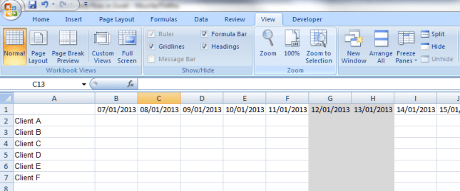
Where is the Freeze Panes button in Excel 2007 and Excel 2010?

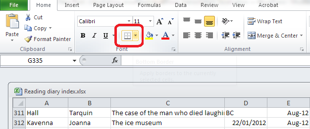
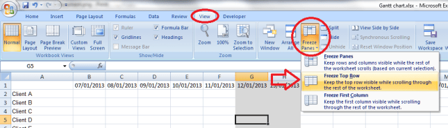
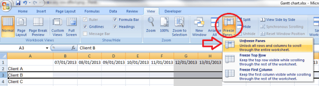
To find the Freeze Panes button, you need to be in the View Tab, then the long Window area. Click on Freeze Panes and you’ll be given three options: Freeze Panes (note, this toggles between Freeze and Unfreeze, as we’ll discover later); Freeze Top Row; and Freeze First Column.

2 freeze top or side

How do I freeze the top row or first column of my spreadsheet?

In a shock move, something that Microsoft Office gives you as a short cut is actually useful! If you click on that Freeze Panes button and select Freeze Top Row or Freeze First Column, it will automatically freeze that row or column for you. This is because the first row and column on a given spreadsheet are likely to be the ones where you’ve inserted your headers.

Click on one of these buttons and you’ll freeze just that row or column. Freeze the top row, scroll down thousands of rows, and that top row will still be on show. Hooray!

BUT: this will only freeze one of those two areas. Want to freeze the spreadsheet so it shows more than just the first row or column? Read the next three sections.

BUT (2): this will only allow you to freeze the row or the column. If you, like me, want to freeze both a row and a column, scan down to the section titled Can I freeze a row and a column at the same time?

How do I freeze a particular row of my spreadsheet?

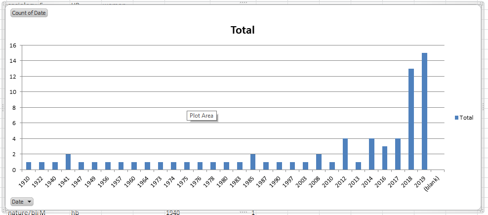
Say, for example, you’ve got a double row of headers, or you’ve inserted a graph at the top of your spreadsheet that you want to be able to see as you scroll down. This is where you need to be able to select the point at which the spreadsheet freezes.

Here’s where it gets a tiny bit tricky (but you’ll save this post so you remember).

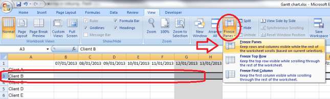
Click on the row BELOW the point at which you want to freeze the spreadsheet. Not the row you want to freeze, the one below it. In this example, we’re highlighting Row 3 in order to freeze Rows 1 and 2.

Once you’ve highlighted the correct row, by clicking on the 3 in the left hand margin in this case (you can see that it’s become darker, with a line around it), click on the Freeze Panes button and select the Freeze Panes option.

3 freeze any row

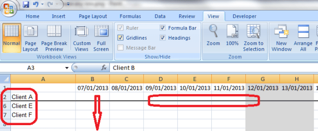
Your spreadsheet is now frozen at the bottom of Row 2. If you scroll down the page, you will notice that Rows 3 and onwards start to disappear, and a horizontal black line appears at the point of freezing.

Now you can scroll down as far as you like, and Rows 1 and 2 will always be visible at the top of the screen:

Effect of freezing any row

How do I unfreeze a row or column?

Once you go to do something else with freezing, you will notice that the Freeze Panes option has changed to read Unfreeze Panes. This is because you can only do one Freezing action at a time. If you decide that you want to freeze a column instead, or want to practise doing that, you need to click the Freeze Panes button then select the Unfreeze Panes option first.

Note: you don’t need to have anything highlighted to click this. It will unfreeze anything you’ve previously frozen.

4 unfreeze panes

Oh, and you can freeze a column and row at the same time, as we’ll learn in a few moments.

How do I freeze a particular column of my spreadsheet?

If you want to freeze a particular column of your spreadsheet, you do it in the same way as you froze the particular row.

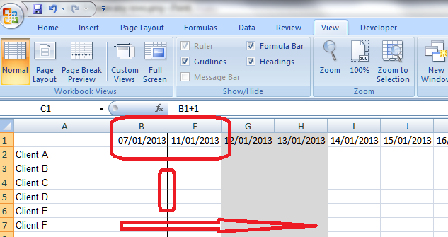
But in this case, you need to highlight the column one to the RIGHT of the column you wish to freeze. In the example below, we want to freeze at Column B, so we highlight Column C (by clicking on the C at the top of the column). Again, click the Freeze Panes button then select the Freeze Panes option.

5 freeze any rows

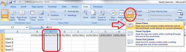
Now, if you scroll across the document, Columns A and B will remain visible, and a thick black line will mark where the freezing has taken place:

5 freeze any rows effect

Can I freeze a row AND a column at the same time?

Sometimes you might want to freeze both the top row and the first column of your spreadsheet. For example, I want to be able to see my list of clients, however many dates come across the page, and my dates in the top row, however long my list of clients becomes.

We’ve already learnt how to freeze just the top row or just the first column (see above), but as you might have realised,  you can’t do both – if you go back to the menu to do the second one, it just tells you to Unfreeze the panes first.

Here’s  how you do it:

Highlight the cell ONE DOWN and ONE TO THE RIGHT of the row and column you want to freeze. It’s just like freezing rows or columns. In this case, think of the cell nestling in the angle formed where the row and column you want to freeze meet. Here, we want to freeze Row 1 and Column A so that they are always visible. So we highlight the point at which Row 2 meets Column B.

6 freeze row and columnt

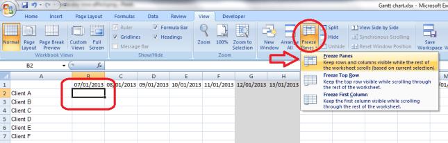
Using the same procedure to freeze the panes (Freeze Panes button, Freeze Panes option), we have now frozen Row 1 and Column A. If we scroll both down and across, Row 1 with the dates and Column A with the client names are still visible.

6 freeze row and column effect

Yes, Column A will scroll and the top will slide up and disappear temporarily, and yes, the dates in Row 1 will disappear as we scroll across, but the basic principle holds good:  we can see Row 1 and Column A, however much we move around the spreadsheet.

We’ve learned how to freeze rows, columns and rows plus columns today. I hope you’ve found this useful.

If you have found this article useful, please share it using the buttons below, and leave me a comment!

Related posts: How to print out the header row on every page

This is part of my series on how to avoid time-consuming “short cuts” and use Microsoft Office in the right way to maximise your time and improve the look of your documents.

Please note, these hints work with versions of Microsoft Excel currently in use – Excel 2003, Excel 2007 and Excel 2010, all for PC. Mac compatible versions of Word should have similar options. Always save a copy of your document before manipulating it. I bear no responsibility for any pickles you might get yourself into!

Find all the short cuts here

 
16 Comments

Posted by on January 9, 2013 in Errors, Excel, New skills, Short cuts, Writing


Tags: , , , , , , ,