It was time to create a new Gantt chart for myself to keep my various projects under control, and yet again I had forgotten how to freeze the columns and rows in the way I like. So I created this post to help myself – and you!
What is “freezing” rows and columns?
When you freeze a row or column in an Excel spreadsheet, you make sure that it’s on display however much you scroll down or across your document.
So, if you have a row of dates as a heading along the top or a column of customer names down the side, and your document becomes longer or wider than the screen on which you are viewing it, you can keep those columns and rows visible, instead of having to scroll up and down and backwards and forwards to find your headings.
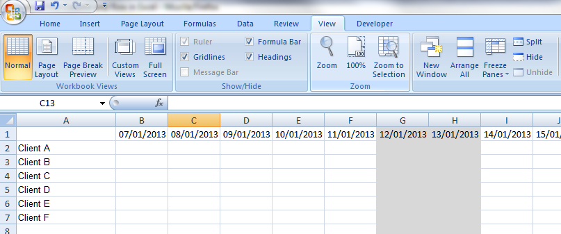
For example, in the Gantt chart that records my work projects, I need to be able to see the dates and client names all the time, however large my document becomes:
Where is the Freeze Panes button in Excel 2007 and Excel 2010?
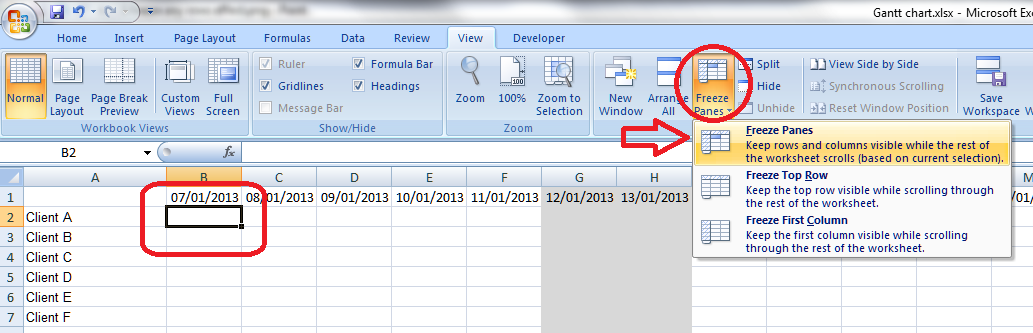
To find the Freeze Panes button, you need to be in the View Tab, then the long Window area. Click on Freeze Panes and you’ll be given three options: Freeze Panes (note, this toggles between Freeze and Unfreeze, as we’ll discover later); Freeze Top Row; and Freeze First Column.

How do I freeze the top row or first column of my spreadsheet?
In a shock move, something that Microsoft Office gives you as a short cut is actually useful! If you click on that Freeze Panes button and select Freeze Top Row or Freeze First Column, it will automatically freeze that row or column for you. This is because the first row and column on a given spreadsheet are likely to be the ones where you’ve inserted your headers.
Click on one of these buttons and you’ll freeze just that row or column. Freeze the top row, scroll down thousands of rows, and that top row will still be on show. Hooray!
BUT: this will only freeze one of those two areas. Want to freeze the spreadsheet so it shows more than just the first row or column? Read the next three sections.
BUT (2): this will only allow you to freeze the row or the column. If you, like me, want to freeze both a row and a column, scan down to the section titled Can I freeze a row and a column at the same time?
How do I freeze a particular row of my spreadsheet?
Say, for example, you’ve got a double row of headers, or you’ve inserted a graph at the top of your spreadsheet that you want to be able to see as you scroll down. This is where you need to be able to select the point at which the spreadsheet freezes.
Here’s where it gets a tiny bit tricky (but you’ll save this post so you remember).
Click on the row BELOW the point at which you want to freeze the spreadsheet. Not the row you want to freeze, the one below it. In this example, we’re highlighting Row 3 in order to freeze Rows 1 and 2.
Once you’ve highlighted the correct row, by clicking on the 3 in the left hand margin in this case (you can see that it’s become darker, with a line around it), click on the Freeze Panes button and select the Freeze Panes option.

Your spreadsheet is now frozen at the bottom of Row 2. If you scroll down the page, you will notice that Rows 3 and onwards start to disappear, and a horizontal black line appears at the point of freezing.
Now you can scroll down as far as you like, and Rows 1 and 2 will always be visible at the top of the screen:

How do I unfreeze a row or column?
Once you go to do something else with freezing, you will notice that the Freeze Panes option has changed to read Unfreeze Panes. This is because you can only do one Freezing action at a time. If you decide that you want to freeze a column instead, or want to practise doing that, you need to click the Freeze Panes button then select the Unfreeze Panes option first.
Note: you don’t need to have anything highlighted to click this. It will unfreeze anything you’ve previously frozen.

Oh, and you can freeze a column and row at the same time, as we’ll learn in a few moments.
How do I freeze a particular column of my spreadsheet?
If you want to freeze a particular column of your spreadsheet, you do it in the same way as you froze the particular row.
But in this case, you need to highlight the column one to the RIGHT of the column you wish to freeze. In the example below, we want to freeze at Column B, so we highlight Column C (by clicking on the C at the top of the column). Again, click the Freeze Panes button then select the Freeze Panes option.

Now, if you scroll across the document, Columns A and B will remain visible, and a thick black line will mark where the freezing has taken place:

Can I freeze a row AND a column at the same time?
Sometimes you might want to freeze both the top row and the first column of your spreadsheet. For example, I want to be able to see my list of clients, however many dates come across the page, and my dates in the top row, however long my list of clients becomes.
We’ve already learnt how to freeze just the top row or just the first column (see above), but as you might have realised, you can’t do both – if you go back to the menu to do the second one, it just tells you to Unfreeze the panes first.
Here’s how you do it:
Highlight the cell ONE DOWN and ONE TO THE RIGHT of the row and column you want to freeze. It’s just like freezing rows or columns. In this case, think of the cell nestling in the angle formed where the row and column you want to freeze meet. Here, we want to freeze Row 1 and Column A so that they are always visible. So we highlight the point at which Row 2 meets Column B.
Using the same procedure to freeze the panes (Freeze Panes button, Freeze Panes option), we have now frozen Row 1 and Column A. If we scroll both down and across, Row 1 with the dates and Column A with the client names are still visible.

Yes, Column A will scroll and the top will slide up and disappear temporarily, and yes, the dates in Row 1 will disappear as we scroll across, but the basic principle holds good: we can see Row 1 and Column A, however much we move around the spreadsheet.
We’ve learned how to freeze rows, columns and rows plus columns today. I hope you’ve found this useful.
If you have found this article useful, please share it using the buttons below, and leave me a comment!
Related posts: How to print out the header row on every page
This is part of my series on how to avoid time-consuming “short cuts” and use Microsoft Office in the right way to maximise your time and improve the look of your documents.
Please note, these hints work with versions of Microsoft Excel currently in use – Excel 2003, Excel 2007 and Excel 2010, all for PC. Mac compatible versions of Word should have similar options. Always save a copy of your document before manipulating it. I bear no responsibility for any pickles you might get yourself into!
Find all the short cuts here …


Andrew
March 6, 2014 at 9:59 pm
Hi, I was interested in doing something similar, but I don’t know if Excel is capable of it. I’m trying to test out an idea, and I have about 15 word lists (each about 1000 words, sorted by syllables, from 1 to about 5), and I’d like to see them all side by side in their own columns. The capability that I’d like to have is the ability to scroll through the individual columns without affecting the others. I’d use Excel, but you can only freeze certain columns and then the unfrozen ones all move together, but I’d like something that resembles 15 wheels, all of which can be turned independently of one another. Is there a program out there that already does this?
LikeLike
Liz at Libro
March 6, 2014 at 10:58 pm
A fascinating question – thank you! Unfortunately, I don’t think this can be done in Excel. I consulted with Mr Libro, too, who is an expert in Excel, and he says no. If you do find out how to do it, then do pop back here and share!
LikeLike
Andrew
March 7, 2014 at 11:59 pm
Ah, I see, well thanks anyways. Do you or Mr. Libro know any other alternatives perhaps? Without opening up 15 notepad documents side by side lol?
LikeLike
Liz at Libro
March 8, 2014 at 7:14 am
A solution we’ve come up with is to use Microsoft Access: put your words into columns into the relational database and then create the form on top of it with 15 text boxes in a row: you should then be able to scroll through the results in each text box using the down arrow in order to get what I presume you want, different combinations of words across the page. I hope that helps. More detail on exactly how you can do that, I can’t give you, but that should give you enough ammunition to approach an Access expert. The other option is to commission someone to write you a custom bit of software, which is actually something Mr. Libro can do, so get in touch via the Contact Me page if you’d like to go down that route. Do drop by and let us know what ensues anyway!
LikeLike
Andrew
March 8, 2014 at 8:00 pm
Oh, but doesn’t that mean I’ll only be able to see essentially one word at a time in each column? The reason I’d like to see all 15 columns side by side is to facilitate the creative process, because the columns each stand for a vowel sound, and I wanted to use this to for my rapping hobby lol. The goal isn’t so much to create a string of 15 words but to just be able to scroll through each of the columns until my brain hopefully makes a connection between the words in at least some of the columns. Will your method work for that too?
LikeLike
Y. O'Connor
July 16, 2014 at 5:25 pm
You are Awwwwesoooome!!!. I have been searching for how to freeze both a row AND a column w/ no luck until now. Thank you soooo much.
LikeLike
Liz at Libro
July 17, 2014 at 6:01 am
You’re welcome! Glad I could help, and thanks for taking the time to comment.
LikeLike
Irene
January 28, 2015 at 9:11 pm
Thanks for this post. I must be really tired because this is so simple. I must have been clicking on the wrong thing, obviously. sigh Wasted time trying to figure it out myself, until I decided to get help and found your post! So thank you again for the reminder. : )
LikeLike
Liz Dexter
January 30, 2015 at 9:43 pm
Glad I could help!
LikeLike
jeanette
April 27, 2015 at 3:34 pm
When I click on the freeze panes button, it gives me the drop down list, but the only options are a. unfreeze panes b. freeze row or c. freeze column. it doesn’t give me a ‘freeze panes’ option, where I can freeze both column and row together. Clicking on the freeze panes button itself does nothing but give me the drop down list
LikeLike
Liz Dexter
April 29, 2015 at 1:58 pm
Thanks for your question. Click on unfreeze panes, then click anywhere on the spreadsheet, then start again and it should work for you. You’ve frozen something somewhere and you need to unfreeze that first.
LikeLike